Magnetografia- Polarimetria solare

 Solar magnetography - polarimetry

 Fulvio  Mete- Roma  

 fulvio_mete@fastwebnet.it

  19 marzo 2017

Appassionato di astronomia dall’età di otto anni,Fulvio Mete ha dedicato buona parte della sua vita a questa sua passione, integrando le conoscenze di astronomia con quelle di fisica, informatica,  meccanica.Da quasi vent’ anni si occupa di spettroscopia astronomica, ha diretto il Settore di Ricerca UAI di Spettroscopia, ha svolto e svolge numerose iniziative di ricerca, quali spettroscopia di nove e supernove, ,spettroeliografia, magnetografia solare, imaging in IR vicino.Ha, altresì, organizzato numerosi eventi di livello nazionale in tale settore, quali i Seminari di Spettroscopia di Asiago e di Arcetri, e molti altri di minore livello.Ha pubblicato articoli su riviste commerciali di divulgazione astronomica (Coelum, Nuovo Orione, Astronomia UAI), nonché articoli in inglese e francese su testi stranieri.Ha partecipato con proprie relazioni a numerosi Convegni e Congressi di astronomia.Ha costruito e costruisce da autodidatta strumenti per la osservazione e ripresa spettroscopica del sole e degli oggetti del cielo profondo, alcuni dei quali hanno carattere di unicità a livello nazionale.

Le osservazioni Zeeman del 2017: macchie più piccole e procedure più rigorose

The Zeeman observations of 2017: smaller sunspot and stricter procedures

L'articolo è il seguito di un analogo lavoro  (il primo) svolto nel 2016, visionabile al link:

http://www.lightfrominfinity.org/Effetto%20Zeeman%20e%20magnetografia%20solare/Effetto%20Zeeman%20e%20magnetografia%20solare%202016.pdf

Premessa:

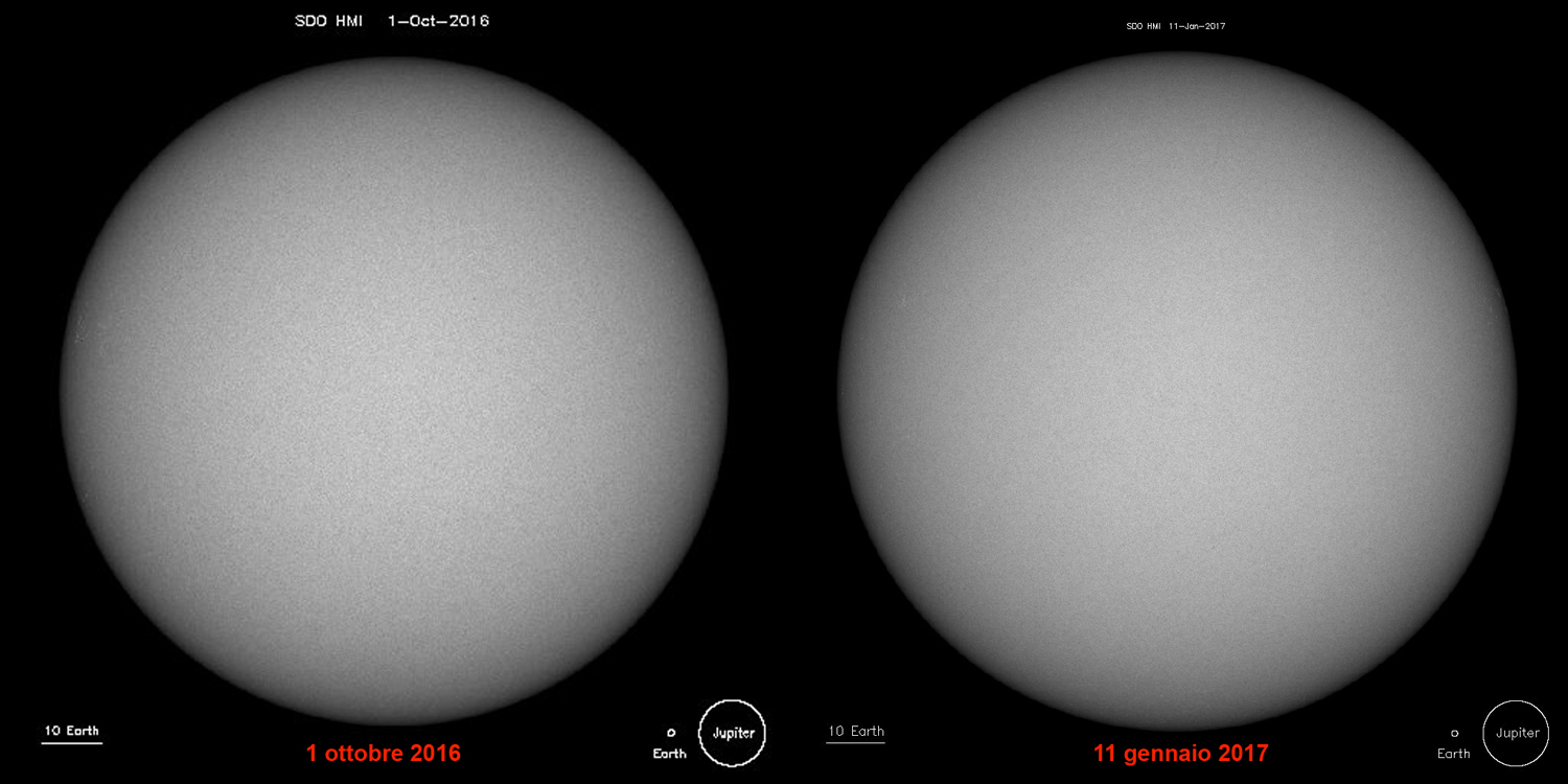
Pur tenendo conto che il ciclo 24 si avvia verso il minimo nel 2019, dal 1 ottobre 2016 sino a metà gennaio 2017, il sole ha presentato l’aspetto indicato nella  foto allegata (fonte SOHO-MDI),un disco totalmente privo di macchie in zona fotosferica e di scarsissima attività a livello cromosferico.Sono stati ben 3 mesi e mezzo, un periodo significativamente lungo di inattività.Fortunatamente la seconda metà del 2017 sembra aver segnato una certa inversione di tendenza, con alcune macchie di notevole estensione, seppure comunque inferiori a quelle dei precedenti cicli 22 e 23.

Premise:

Even taking into account that the 24 cycle is moving towards the minimum in 2019, from  October 1st 2016 until mid-January 2017, the sun has presented the appearance shown in the following picture (source SOHO-MDI),a disk totally free from sunspots in photospheric area and with very low-level of cromospheric activity: were as many as 3 and a half months, a period of considerable long low activity.Fortunately the second half of the year 2017 seems to have marked a trend reversal, with some sunspots of noticeable extension, although lower than those of previous cycles 22 and 23.

Revisione della procedura

L’esperienza del 2016 è stata fondamentale per la comprensione delle potenzialità e dei limiti del sistema da me concepito per la misurazione dei campi magnetici delle macchie solari per mezzo dell'effetto Zeeman inverso. La vera novità rispetto alle precedenti osservazioni è stato l’uso di una fenditura  fissa da 5 micron, acquistata da Edmund Optics ai primi di gennaio 2017: e devo dire che questa è stata un’arma vincente, in quanto mi ha fatto ottenere un notevole guadagno in risoluzione spettrale, che ha toccato R = 100000 in condizioni di seeing buono e con l’applicazione del solito filtro wavelet.La fenditura fissa, lavorata al laser di precisione, ha fatto diminuire le potenziali fonti di errore dovute alla fenditura stessa, circoscrivendo gli errori al seeing diurno ed al software di elaborazione dello spettro e di determinazione dei centri delle righe Zeeman. L’uso di una fenditura molto stretta, se da un lato permette di accostarsi alla misura di macchie di minore estensione e quindi allarga notevolmente il campo di usabilità dei miei strumenti, postula tuttavia l’uso di una procedura più rigorosa, per evitare errori dovuti al seeing ed al software di gestione.

1-     Errori dovuti al seeing

Gli errori dovuti al seeing possono ritenersi controllati in modo sufficiente dallo stacking di circa 300- 500 frames singoli, che vengono mediati tra loro.

2-Errori dovuti al software di conversione dello spettro e di determinazione dei centri riga.

L’uso di un filtro wavelet per individuare le righe splittate è quasi obbligato, ma questa operazione ha tuttavia il prezzo  di aumentare notevolmente il rumore dello spettro bidimensionale e del profilo relativo.Del resto la semplice valutazione dei centri riga in pixel sullo spettro bidimensionale,con la relativa differenza da moltiplicare per la dispersione in Angstrom è per forza di cose imprecisa.Errori di centesimi di Angstrom, che potrebbero sembrare insignificanti possono in realtà far cambiare in modo notevole il risultato della misura: l’errore di 1 pixel nel centro riga alla dispersione di 0.021 A/pixel è infatti pari ad un valore 0.0105 A e di ben 236 Gauss nel valore di B :del resto, come si è detto, Visual Spec e gli altri software analoghi sono stati concepiti per misurare righe dritte e non fortemente inclinate tra loro in misura opposta (a parte la loro sovrapposizione all’ombra molto scura della macchia): è quindi assolutamente necessario definire un sistema di valutazione degli errori del software di conversione.Sia ben chiaro che si entra in un campo assolutamente precluso agli amatori,nel quale ogni passo ulteriore è una sfida.Del resto la potenzialità di strumenti come VHIRSS e Solarscan  ne esce notevolmente estesa ed enfatizzata nei risultati.

le linee guida delle mie osservazioni di misurazione dei campi magnetici delle macchie solari, alla luce dei necessari miglioramenti, possono così sintetizzarsi:

1-     Acquisizione di 3 o più filmati dello spettro della riga interessata e della macchia di circa 400- 500 frames ad un frame rate di 1/15 di sec (o superiore).Se possibile, ma non sempre lo è, cercare di operare una flat.La camera di acquisizione deve avere una risoluzione e sensibilità sufficiente, ma direi  un sensore di almeno ½ di pollice e 1280 x 1024 pixel di risoluzione.Scegliere il migliore filmato, quello in cui la separazione della riga è meglio visibile.

2-     Media dei frames ed estrazione di uno spettro mediato con un leggero filtro wavelet (che ovviamente dovrà essere sempre lo stesso per tutte le osservazioni del genere).L’operazione di media consente di abbattere in misura notevole gli effetti del seeing.Correzione dello spettro bidimensionale per lo slant o smile con IRIS od altro programma equivalente.

3-     Estrarre il profilo dello spettro.Per fare ciò è necessario che il binning sia quanto più stretto possibile (pochi pixel) e centrato sulla striscia scura che attraversa lo spettro, l’ombra della macchia; ciò al fine di limitare al massimo l’errore del programma di estrazione del profilo spettrale che opera su righe Zeeman oblique rispetto al piano spettrale.Il profilo  andrà poi calibrato in lunghezza d’onda , corretto per la risposta e normalizzato.

4-     Definire provvisoriamente ed in via di massima i centri delle righe verso il blu e   verso il rosso sullo spettro bidimensionale con un programma di fotoritocco per fotografia astronomica (Maxim DL, Astroart,Iris, etc),quindi farne la differenza in pixel, moltiplicare la stessa per la dispersione dello spettro per ottenere la differenza in Angstrom, che servirà come dato di orientamento e controllo per quella più precisa operata sul profilo spettrale.

5-     Operare sul profilo spettrale per ottenere i centri riga in Angstrom (in Visual Spec può essere utile”allargare” il profilo lungo l’asse x con la rotellina del mouse) per rendere meglio visibili i centri riga.Può inoltre essere utile, per operare la selezione necessaria per definire il centro riga, individuare con esattezza il continuo,che in caso di spettro rumoroso è impreciso. In tal caso VSpec aiuta con la procedura di definizione del continuo automatico, che applica un filtro Spline al continuo stesso.

6-     Una volta delimitati i centri delle righe Zeeman splittate si operano tre misure del loro valore in Angstrom e si mediano tra loro,facendo poi la differenza dei  risultati.Si ripete l’operazione almeno per tre volte, ottenendo tre valori della reciproca distanza tra i due centri riga dai quali si ottiene la media finale (che divisa per due darà il valore di D lambda per il calcolo di B)mentre la semidispersione massima o la deviazione standard (nel caso di misure oltre le tre) di tale media ,sempre divisa per 2, definirà l’errore della misura.Tale procedura potrà sembrare macchinosa, ma è il minimo da fare per ottenere valori di una sufficiente precisione  in considerazione della strumentazione amatoriale usata.

        Revision and improvements in the procedure of measurement of solar sunspot magnetic fields

The experience of 2016 has been fundamental to the understanding of the potential and limitations of the system I designed to measure the magnetic fields of sunspots. The real novelty compared to previous observations was the use of a fixed 5 micron slit, purchased by Edmund Optics in early January and I can say that this was a winning choice, because I did get a significant gain in spectral resolution, which reached R = 100,000 in good seeing conditions and with the application as usual, of a wavelet filter. The fixed slit, machined by a precision laser, decreased potential sources of error due to the slit itself, circumscribing errors to daytime seeing, and to the spectrum processing software and determination of the Zeeman lines centers.

The use of a very narrow slit, if from one side allows to approach to the measurement of sunspots of smaller extent and thus considerably enlarges the field of usability of my instruments, however, presupposes the use of a more rigorous procedure, to avoid errors due to the seeing and the software.

1- Errors due to seeing

Errors due to seeing can be considered controlled sufficiently by the stacking of about 300- 500 individual frames, which are mediated.

2-Errors due to the spectrum conversion software and the determination of line centers.

The use of a wavelet filter to locate the splitted lines is almost obligatory, but this operation has however the price of greatly increase the noise of the two-dimensional spectrum and the related profile.However, the simple evaluation of the pixels of the line centers in the two-dimensional spectrum, with their difference multiplied by the dispersion in Angstrom is necessarily inaccurate.Errors of hundredth of an Angstrom, that may seem insignificant can actually dramatically change the outcome of the measurement: the error of 1 pixel in the center line is, at dispersion of 0.021 A/pixel equal to 225 Gauss in the measure of B, but conversion software, VSpec and other similar, have been conceived to measure straighten lines, and not inclined ones (apart the uncertainty of their superimposing to the sunspot umbra.Is then mandatory to define a strict procedure per the evaluation of software conversion errors .But you are now entering in a field absolutely precluded to amateurs, in which each step is a further challenge.In every case the potential of instruments like VHIRSS and Solarscan comes out greatly extended and emphasized in the results.

The guidelines of my observations of measurement of solar sunspot magnetic fields,  can be summarized as follows:

 1-Capture three or more  400- 500 frames videos at a frame rate of 1/15 fps (or higher) .You can, but not always so, try to make a flat. The capture camera for acquisition of a movie of the spectrum of the line and the sunspot shall have a sufficient resolution and sensitivity, I would say a sensor of at least ½ inch and about 1280 x 1024 pixels.Choose the better between the video acquired.

2- Median of frames of the video and extraction (with a software as Registax,Iris,Autostakkert, etc) of an average spectrum with a light wavelet filter (which of course will always be the same for all such observations) .Correction of the bidimensional spectrum for the slant or smile with IRIS or other equivalent software.

3- Estract the profile of spectrum: I use Visual Spec, but also others free software do the job (Isis,BASS,etc). This requires that the binning is as tight as possible (a few pixels) and centered on the dark stripe running through the spectrum, the umbra of the sunspot; this in order to minimize the error of the software in the extraction of the spectral profile, considering that  it operates on the Zeeman lines oblique with respect to the spectral plane.The profile will then  be calibrated in wavelength, corrected for the response and normalized.

4- Provisionally define roughly the centers of the lines towards the blue and toward the red with a photo editing program for astrophotography (Maxim DL, Astroart, Iris, etc), then make the difference in pixels, multiply the same for the dispersion of the spectrum to obtain the difference in Angstroms between the two lines, which will serve as a system of guidance and control for the one, more precise,to be operated on the spectral profile.

5- To work on the spectral profile to get the splitted line centers in Angstrom (in Visual Spec can be useful "enlarge" the contour along the x axis with the mouse wheel) to make more visible the lines itself.

It may also be useful to operate the selection necessary to define the center line, to pinpoint the continuous, that in case of noisy spectrum is quite inaccurate: in this case Visual Spec helps with the continuum automatic setting routine, which applies a spline filter to the continuum.

6- Once selected the centers of the two splitted Zeeman lines we will operate three measurements of their values in Angstrom and after the difference between   the median of such values.We’ll repeat the operation for three times, and with the three numbers showing the distance between the two lines we will  make the final median  that is divided by two to get the d lambda for the definition of the magnetic field in Gauss.The half maximum dispersion or standard deviation (in the case of more than three of the median), divided by two, will show the error.

AR 2628- 25 gennaio 2017

Il target

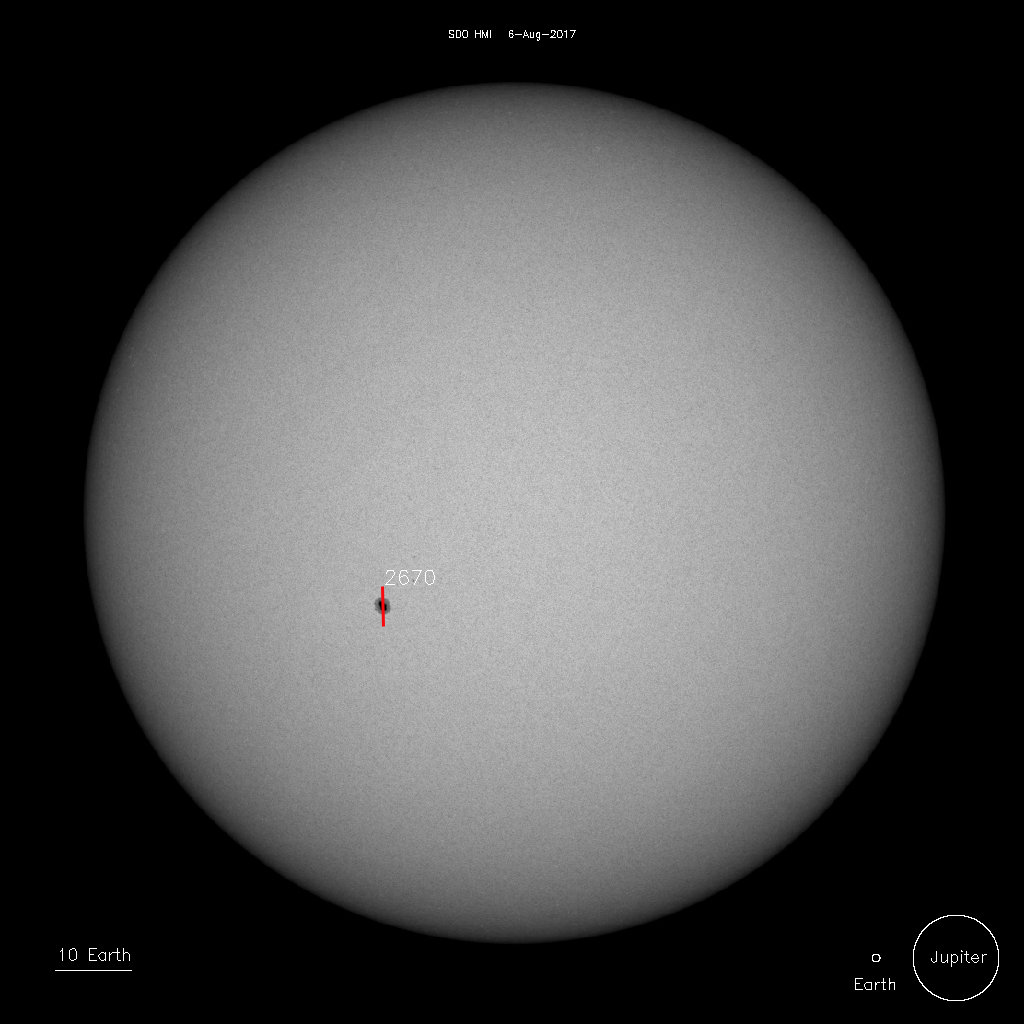
Un minimo segno di ripresa di attività si è avuto nella seconda metà di gennaio 2017, con una macchia di appena discreta estensione, la AR 2628, che ho ritenuto essere un buon campo di prova per testare la nuova fenditura per Solarscan, da soli 5 micron,di cui ho detto in precedenza.Mi aspettavo infatti un miglioramento di risoluzione spettrale tale da poter apprezzare l’effetto Zeeman anche in macchie di modesta estensione come quella in questione.

The target

Minimal signs of recovery of activity has had in the second half of January 2017, with a sunspot of sufficient extension, the AR 2628, that I felt to be a good testing ground to test the new slit for Solarscan,of only 5 microns, I said before.Then I was expecting an improvement in spectral resolution capable to detect the Zeeman effect even in modest extension sunspots  such as the one in question.

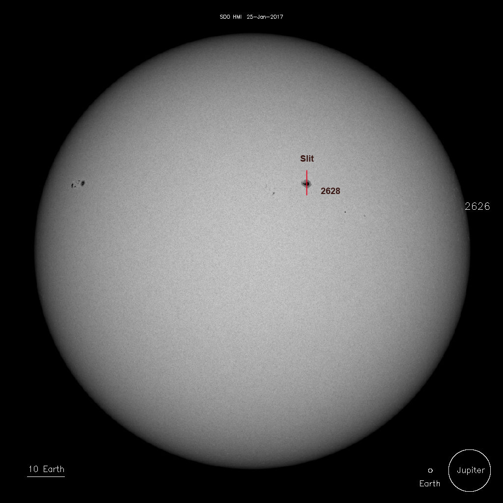
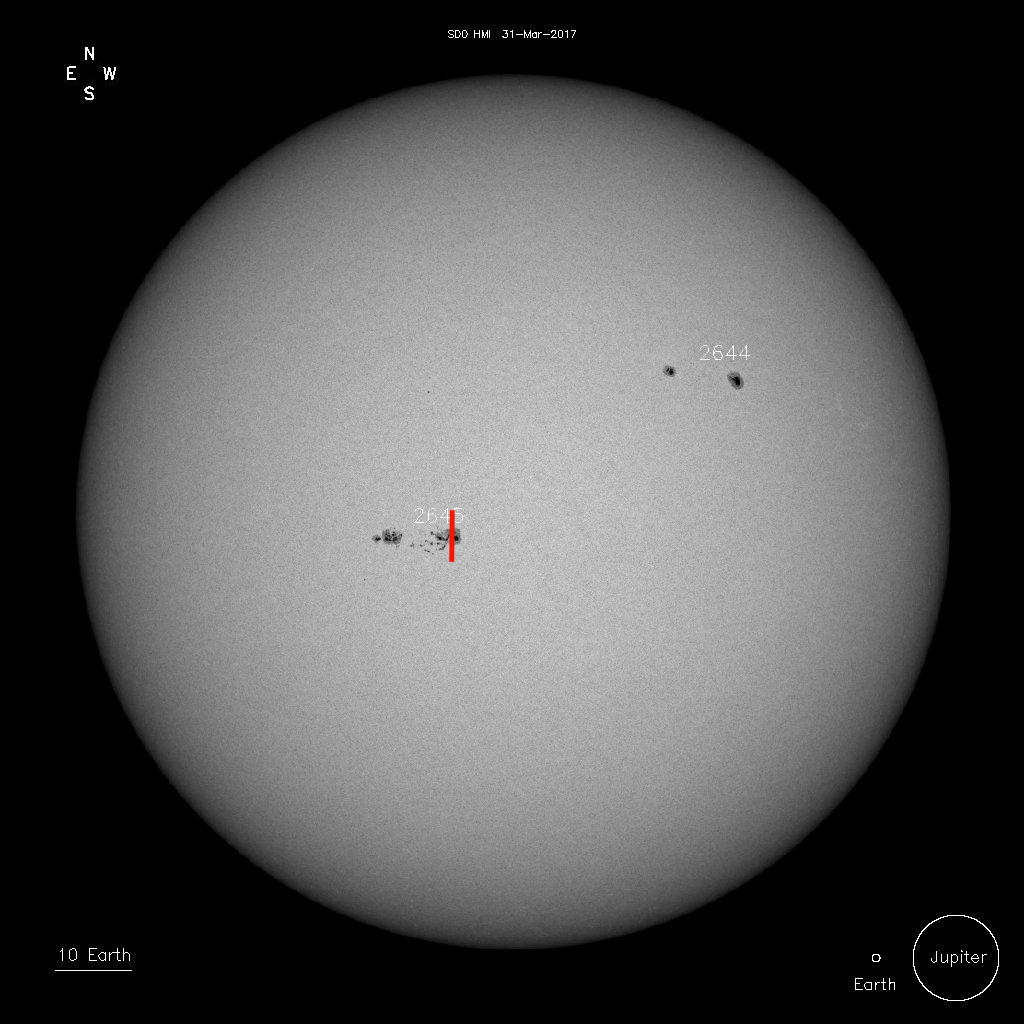
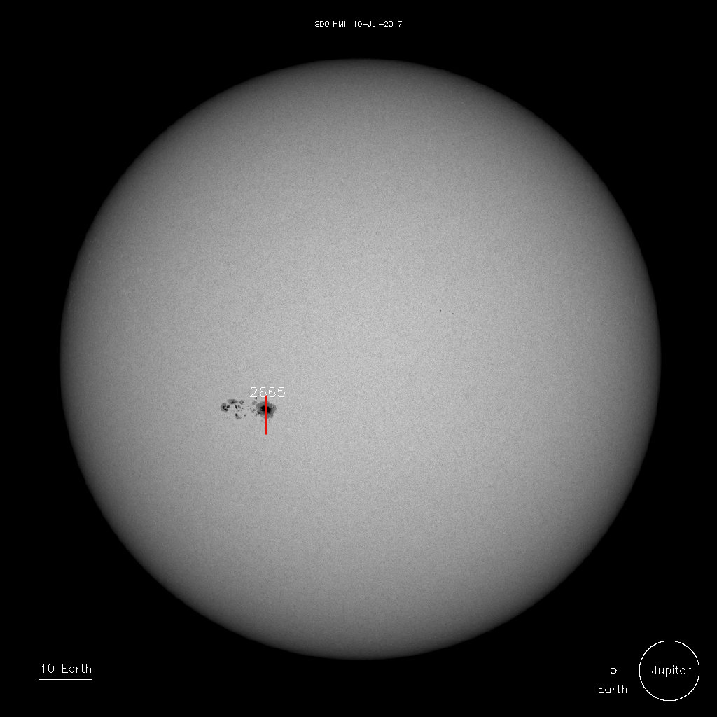
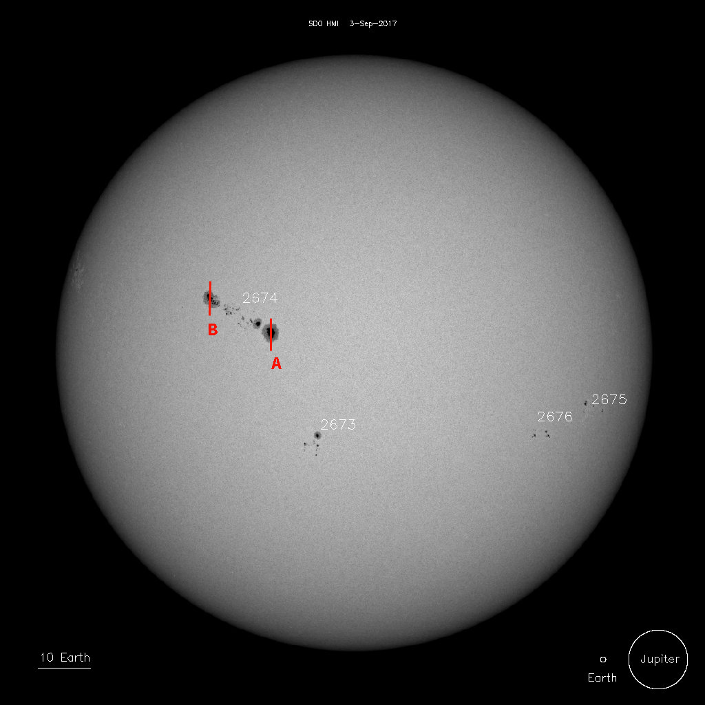
                                                                                                                        L’AR  2628 con la posizione della fenditura il 25 gennaio 2017 (fonte SDO-HMI).

                                                                                                                          AR 2628 with the position of the slit on january, 25, 2017 (source SDO-HMI).

La strumentazione usata

La strumentazione usata è stata quella dei casi precedenti: Lo spettrografo Hires Solarscan sviluppato, su progetto di chi scrive, dalla nota ditta Avalon di Aprilia (RM):Si tratta di uno strumento di alta qualità tecnologica e meccanica completamente automatizzato e remotizzabile, capace di risoluzioni spettrali anche notevolmente superiori a R= 60000 in un peso di 15 Kg e una lunghezza di circa 110 cm, quindi perfettamente gestibile da una sola persona su montature equatoriali di classe media come Losmandy G11 ed Avalon M1.La camera era una  IS DMK 41, con sensore Sony ICX 285 AL da 1280 x 1024 su montatura Losmandy G 11.C’è da dire, a proposito della camera, che, pur avendo recentemente acquistato una DMK 51 da 1600 x 1200, mi è sembrato che la 41 sia più sensibile ed adatta per lavori al limite della strumentazione, come quello in discorso.La vera novità rispetto alle precedenti osservazioni è stato l’uso, come detto, di una fenditura  fissa da 5 micron.La macchia 2628 era infatti poco estesa, ed ho molti dubbi che sarei riuscito a rivelarne l’effetto Zeeman senza l’uso della nuova fenditura.

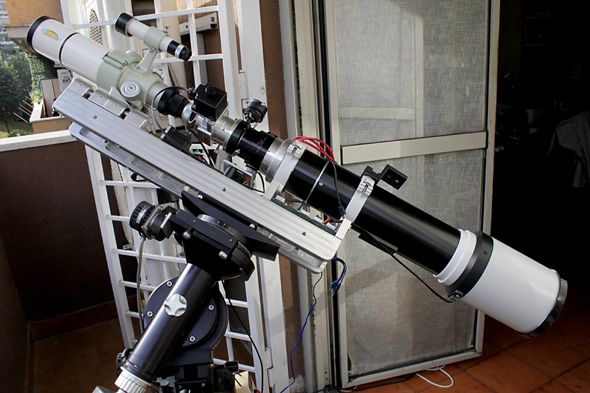
The equipment used

The equipment used was that of the previous cases: The Hires spectrograph Solarscan developped, on my layout, by the known firm Avalon of Aprilia (Rome) capable of remote operation, and a camera DMK 41, with Sony ICX 285 AL sensor 1280 x 1024 on Losmandy G 11 mount.I must say, about the camera, which, although having recently purchased a DMK 51 1600 x 1200, it seemed that the 41 is more sensitive and suitable for work at the limit of the equipment, like the one in topic.The sunspot 2628 was in fact small and I have many doubts that I would be able to reveal the Zeeman effect without the use of the new slit.

L’osservazione

The observation

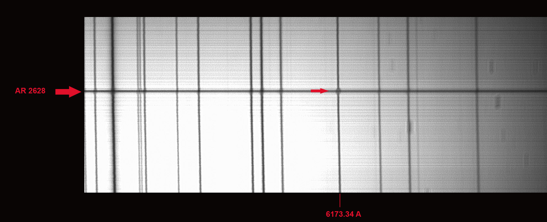
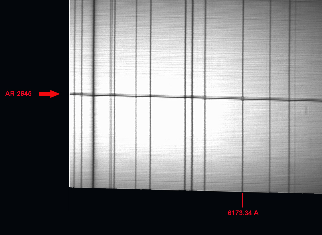
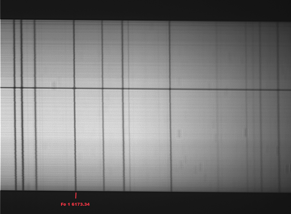
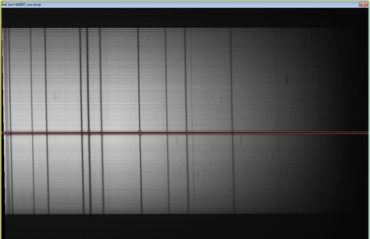
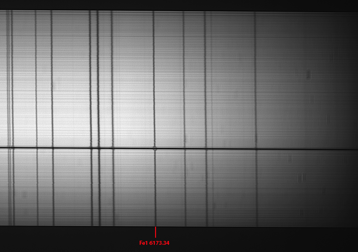
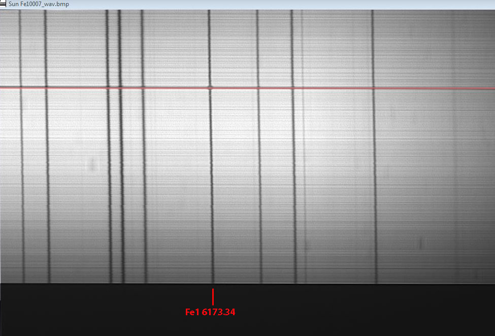
Lo spettro bidimensionale, ottenuto dalla media di ca 300 frames del migliore tra 4 video era il seguente:

The bidimensional spectrum, obtained from the median of 300 frames of the better   of 4 videos was the following:

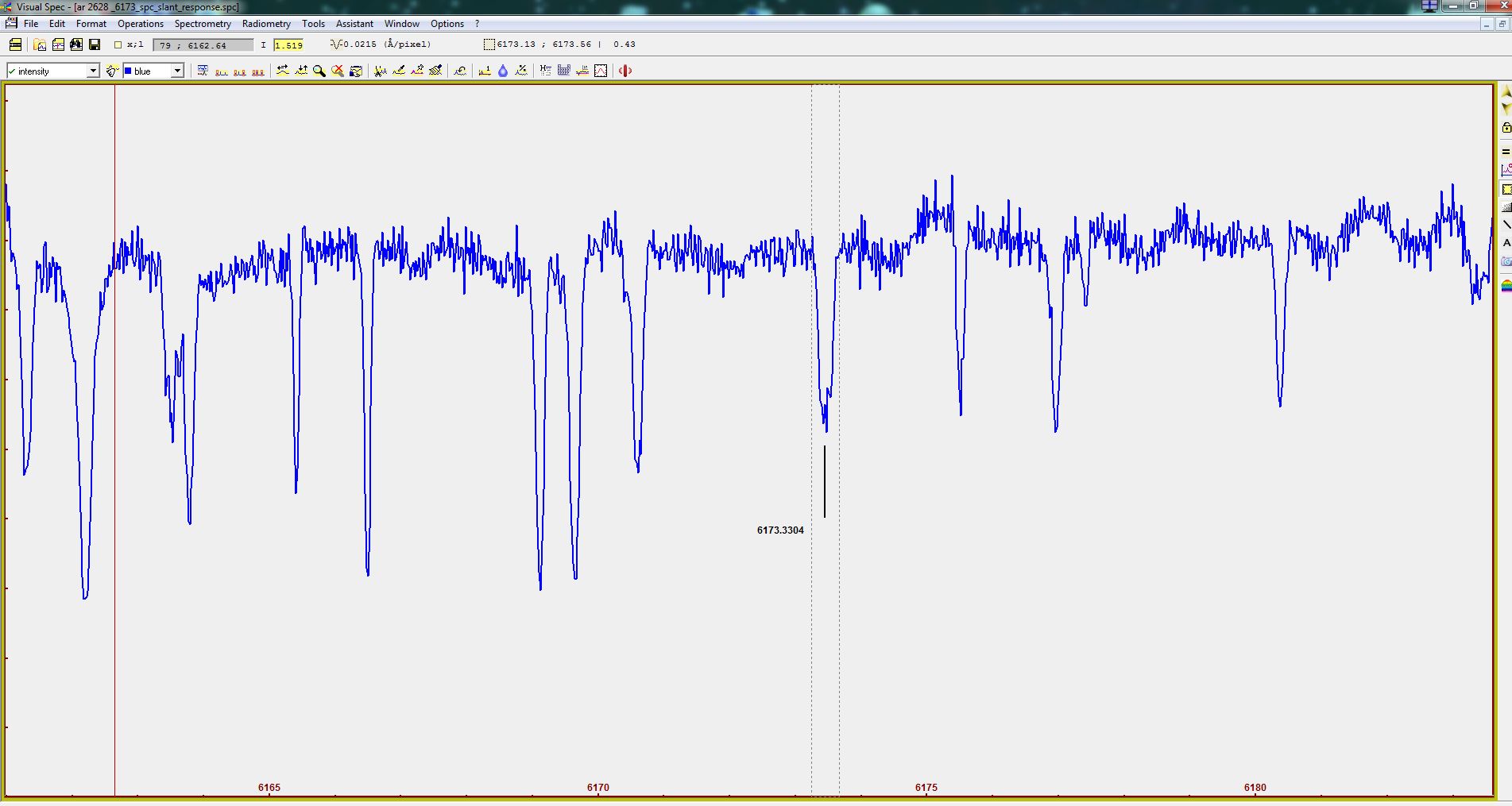
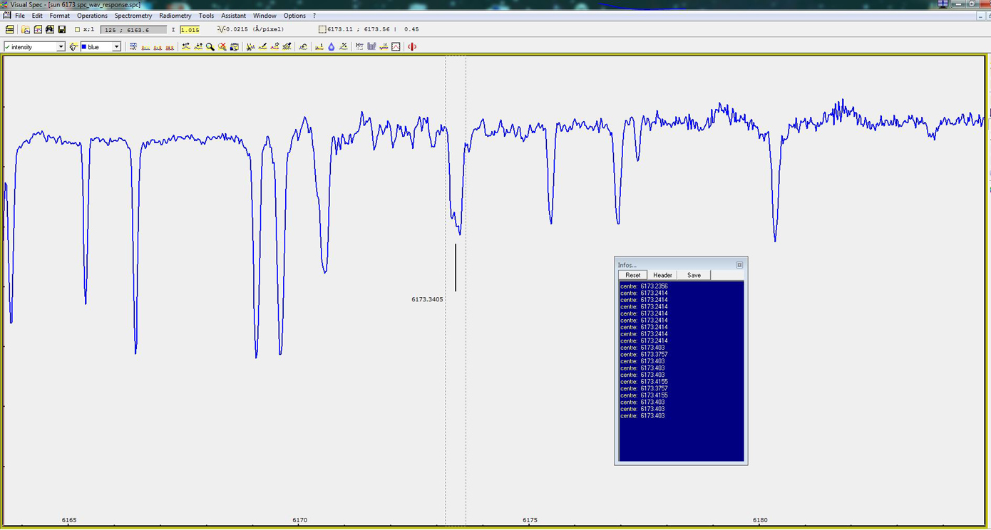
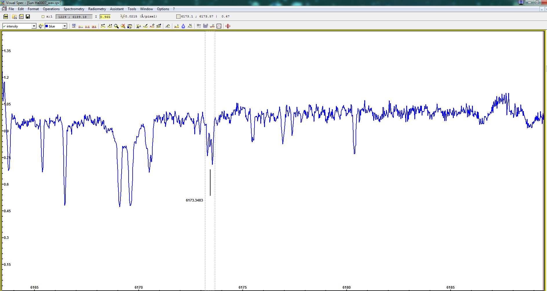
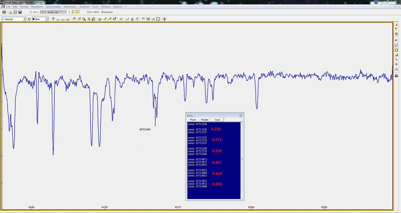
Ed il suo profilo

And its profile

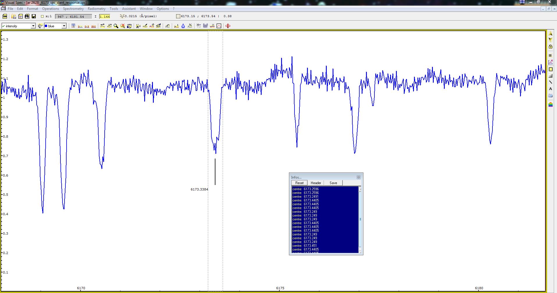
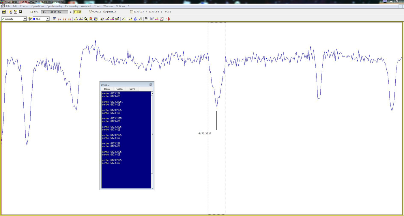
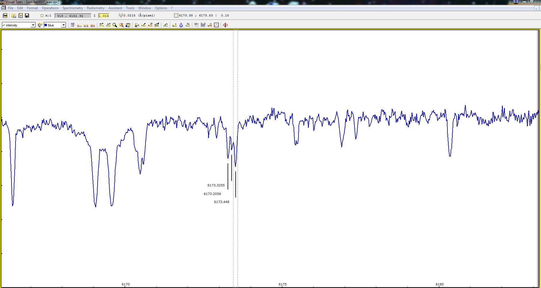
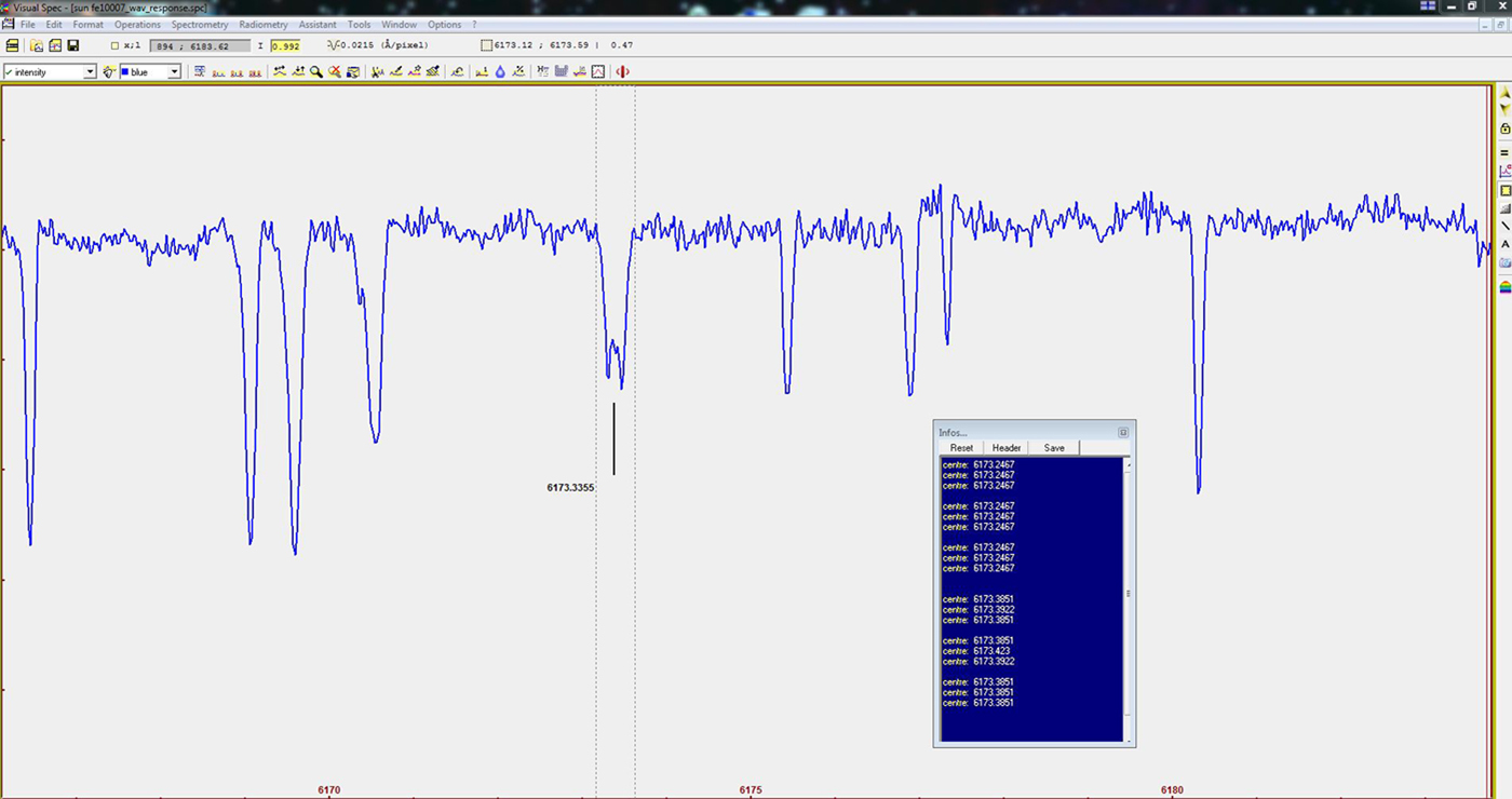
Lo spettro allargato lungo l’asse x per la migliore identificazione dei centri riga splittati e, nel menu a tendina blu,i risultati delle  tre misurazioni (ciascuna a sua volta media di tre).

The spectrum enlarged along x axis to enhance the center of the splitted lines and, in the blue drop down menu, the result of three measures (each in turn composed of three measure)

La procedura descritta, per quanto laboriosa, sembra funzionare abbastanza bene e forniva i seguenti risultati per i centri delle due righe , quella verso la parte blu dello spettro e quella verso il rosso.

The described procedure, although laborious, seems to work quite well, and gave the following results for the two center lines and their differences.

                                                      Ricordando la formula di B citata nel precedente articolo:

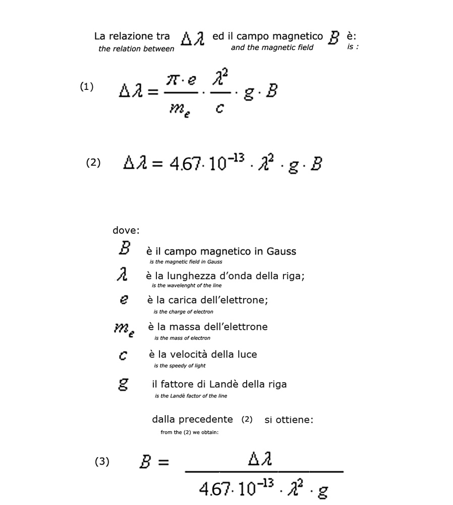
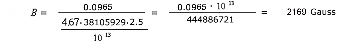
                                              In definitiva è:

Per il calcolo dell’errore statistico sul d lambda ottenuto si è usato il sistema della semi dispersione massima, già usato in precedenza e suffiicientemente affidabile per tre misure; era quindi:

The calculation of statistical error on d lambda was done with the half maximum dispersion method, quite reliable with only three measures, was then:

0.0975-0.0922 /2 = 0.00265

0.00265 x 10 ^13  =  59 Gauss

   444886721

Quindi il valore trovato era :

Then the final value was   :          B=   2169+- 59 Gauss

AR 2638 - 26 febbraio 2017

Il target

Si trattava di una regione attiva limitata e di una macchia piccola, di superficie appena superiore a quella terrestre, la più piccola da me osservata sinora con Solarscan: questo rendeva difficile l’osservazione dell’effetto  Zeeman sulla solita riga del ferro, ma comunque valeva provare.

The target

It was a limited active region and a small sunspot, just above the Earth's surface, the smallest from me so far observed with Solarscan: this made it difficult the observation of the Zeeman effect on the usual iron line, but still worth try.

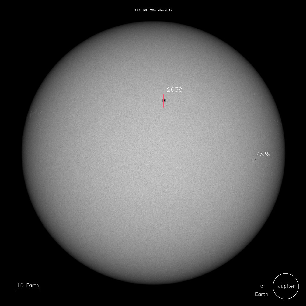
La macchia AR 2638 il 26 febbraio 2017- fonte SDO-HMI

Sunspot AR 2638 on february, 26, 2017 source SDO-HMI

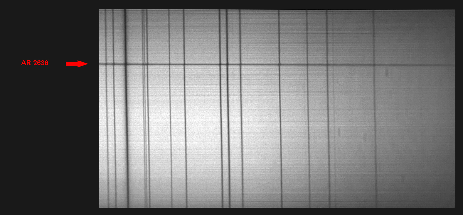
L’osservazione

Lo spettro bidimensionale, ottenuto dalla media di 300 frames su un video di 500.Tale video era stato considerato il migliore di una serie di 4, presi in una giornata di seeing cattivo.

The observation

The two-dimensional spectrum, obtained from the average of 300 video frames of a video of 500.This had been considered the best of a series of 4, taken on a day of bad seeing.

E, di seguito, il profilo spettrale coi centri riga (3 misure per ciascun centro riga x 3 volte)

And, hereunder, the spectral profile with the line centers (three measures for each line center for three times).

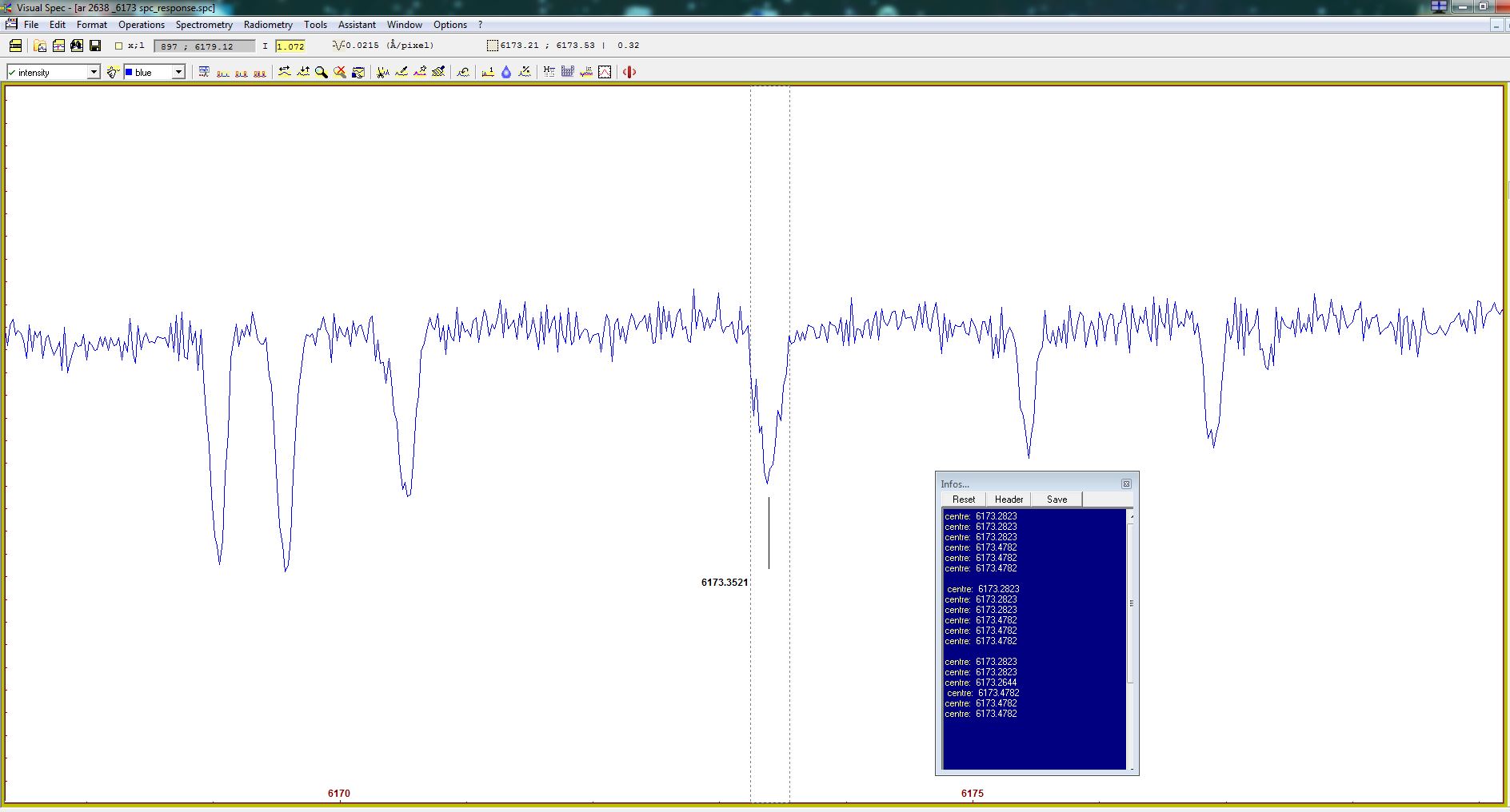
Le differenze delle medie delle  tre misure ed il d lambda sono state rispettivamente pari a:

The difference of the median of the three measures and d lambda were:

Differenza           d lambda

0.1959                  0.0979

0.1959                  0.0979

0.2019                  0.1009

E la loro media pari a

And their median of

 0.1979 A  ; d /lambda di 0.0989

Quindi, applicando la formula precedente:

Then, applying the previous formula:

0.0989 x 10 ^13  =  2223 Gauss

   444886721

E l’errore:

And the error:

0.1009-0.0979/2= 0.0015 A, ovvero:

0.0015 x 10 ^13  =    34 Gauss

   444886721

Quindi B= 2223 +-  34 Gauss

AR 2645 - 31 marzo 2017 

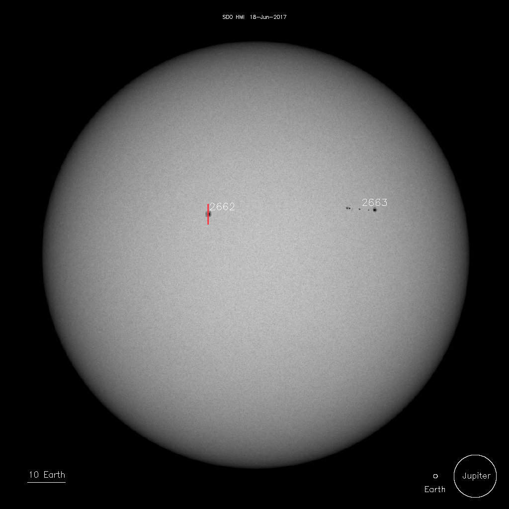
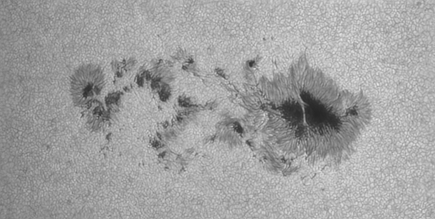
Il target

Si trattava di una regione attiva  formata da un gruppo bipolare con altre piccole macchie con penombra estesa ed ombra piuttosto ridotta, esteso in direzione est-ovest: la fenditura era posta sulla seconda macchia verso ovest.

The target

It was an active region formed by small sunspot, in a bipolar group, with a wide penumbra and small umbra, extended in est-west direction.The slit was put on the second sunspot.

L’osservazione

Lo spettro bidimensionale, ottenuto dalla media di 600 frames su un video di 800.Tale video era stato considerato il migliore di una serie di 3.

 The observation

The two-dimensional spectrum, obtained from the average of 600 video frames of a video of 800.This had been considered the best of a series of 3.

E, di seguito, il profilo spettrale, calibrato come d'uso, coi centri riga (3 misure per ciascun centro riga x 3 volte)

And, hereunder, the spectral profile, calibrated as usual, with the line centers (three measures for each line center for three times).

Le differenze delle medie delle  tre misure ed il relativo d lambda sono state rispettivamente pari a:

The difference of the median of the three measures and related d lambda were:

Differenza           d lambda

0.1545                 0.0772

0.1657                  0.0828

0.1566                  0.0783

E la loro media pari a

And their median of

 0.1589 A  ; d /lambda di 0.0794

Quindi, applicando la formula precedente:

Then, applying the previous formula:

0.0794 x 10 ^13  =  1785 Gauss

   444886721

E l’errore:

And the error:

0.0828-0.0772/2= 0.0028 A, ovvero:

0.0028 x 10 ^13  =    63 Gauss

   444886721

Quindi B= 1785 +-  63 Gauss

  AR 2662 - 18 giugno 2017

Si trattava di una macchia molto piccola, di estensione ridotta (appena poco più del diametro terrestre, come si osserva dall'immagine sottostante (fonte SOHO-MDI).

It was a small sunspot, with a little more extension then the terrestrial diameter, how we can observe in the following image (source SOHO-MDI)

L’osservazione

Lo spettro bidimensionale, ottenuto dalla media di 500 frames su un video di 1000.Tale video era stato considerato il migliore di una serie di 3.Il seeing era  sotto la media per vento.

 The observation

The two-dimensional spectrum, obtained from the average of 500 video frames of a video of 1000.This had been considered the best of a series of 3. The seeing was under the median for wind.

E, di seguito, il profilo spettrale, calibrato come d'uso, coi centri riga (3 misure per ciascun centro riga x 3 volte)

And, hereunder, the spectral profile, calibrated as usual, with the line centers (three measures for each line center for three times).

Le differenze delle medie delle  tre misure ed il relativo d lambda sono state rispettivamente pari a:

The difference of the median of the three measures and related d lambda were:

Differenza           d lambda

                                                                 0.193              0.0965     

                                                                 0.196              0.0980

                                                                0.193               0.0965 

E la loro media pari a

And their median of

 0.194 A  ; d /lambda di 0.097

Quindi, applicando la formula precedente:

Then, applying the previous formula:

0.097 x 10 ^13  =  2180 Gauss

   444886721

E l’errore:

And the error:

0.0980-0.0965/2= 0.00075 A, ovvero:

0.00075 x 10 ^13  =    17 Gauss

   444886721

Quindi B= 2180 +-  17 Gauss

AR 2665 - 10 luglio 2017

Il 7 luglio è apparsa sul disco solare quella che potrebbe essere il gruppo di macchie più esteso dell'anno in corso ,visibile nell'immagine sottostante, fonte  Soho MDI, con l'indicazione della posizione della fenditura .

On july, 7th appeared on the solar disk a sunspot group that can be defined the largest since the beginning of the current year: it is showed in the following image,(source SOHO-MDI) with the position of the slit.

Il componente maggiore del gruppo era caratterizzato nella sua parte centrale da un notevole light bridge, come si può osservare nell'immagine che segue, ottenuta dall'astrofilo  Turi Lo Vecchio il 9 luglio.

The major component, the large sunspot on the right, had on the center of its umbra a noticeable light bridge,as showed in the following image,obtained by  italian amateur astronomer Turi Lo Vecchio on July, 9.

Nel giorno dell'osservazione, il 10 luglio,  caratterizzato da un meteo dal calore eccessivo , con punte di 38°,e da un'alta pressione di matrice africana eccezionalmente stabile poteva mettere a dura prova la stabilità delle fenditura da 5 micron, per cui l'osservazione è stata effettuata alle  8 UT, quando c'erano "solo" 30°.Lo spettro bidimensionale, il migliore di quelli ottenuti da tre video di 600 frames  era il seguente, con lo splitting della riga ben evidente in presenza di un'ombra piuttosto profonda:

The day of the observation, the 10 of july, was characterized by a very stable African high pressure, that gave temperatures up to 38° C, so it was a very hard task not to compromise the stability of the 5 micron slit.For this reason  the observation was carried out at 8 am UT, when the outside temp was "only" 30 °.The bidimensional spectrum, the better of three obtained from the stacking of 600 frames videos, was the following.

 L'alta pressione ed un seeing diurno eccezionalmente  stabile hanno tuttavia reso questa osservazione unica tra quelle da me sinora effettuate, in quanto , per la prima volta nell'anno, nel profilo spettrale dell'ombra calibrato e normalizzato  con VSpec  risultavano nettamente osservabili non solo le due ali dello splitting Zeeman della riga, ma anche quella centrale.Nell'immagine sottostante si osserva l'area di binning operata sull'ombra della macchia.

The high pressure and the hot air had anyway a positive feature: an exceptionally stable daily seeing that, for the first time in the year, in the spectral profile of the sunspot umbra, calibrated and normalized by Visual Spec, were easily observable all the three components of the Zeeman splitting of the 6173 A Fe1 line.In the image is showed the binning area used for the profile.

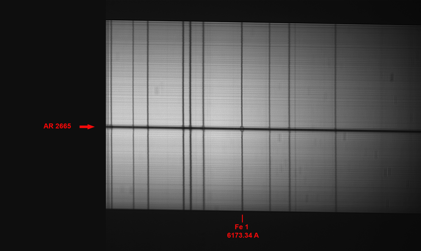
Nell'immagine che segue si osserva il profilo spettrale con le tre cuspidi dello splitting, compresa quella centrale, per la prima volta da me osservata con tale chiarezza.

                                                                In the image that follows, the splitted Zeeman line

 In questo stato di cose, l'individuazione precisa del centro riga e delle cuspidi laterali poteva essere effettuato direttamente con l'apposita routine "label" di VSpec  e la individuazione del d lambda diveniva estremamente semplice, in quanto bastava operare la media degli  scostamenti delle due cuspidi laterali da quella centrale, tuttavia, ho deciso anche stavolta di ricorrere alla procedura standard seguita nei casi precedenti

The precise definition of the center line and the d lambda was then easily  done by the routine "label" of VSpec.Anyway, I decided , also this time, to use the standard procedure applied to the previous cases.

Le differenze delle medie delle  tre misure delle due cuspidi a lato del centro riga ed il relativo d lambda sono state rispettivamente pari a:

The difference of the median of the three measures and related d lambda were:

Differenza           d lambda

  0.2408                  0.1204

  0.2396                  0.1198

  0.2413                 0.1206

E la loro media pari a

And their median of

 0.240 A  ; d /lambda  0.120 A

C'è da dire che il d lambda trovato coincide con quello ricavato dalla routine "label" di VSpec (6173.20+0.12=6173.32 +0.12= 6173.44)

Must say that the d lambda found is almost the same of the one resulting from the routine "label" of VSpec (6173.20+0.12=6173.32 +0.12= 6173.44).

Quindi, applicando la formula precedente:

Then, applying the previous formula:

0.120 x 10 ^13  =  2697 Gauss

   444886721

E l’errore:

And the error:

0.1206-0.1198/2= 0.0004 A, ovvero:

0.0004 x 10 ^13  =    9 Gauss

    444886721

Quindi B= 2697 +-  9 Gauss

Due considerazioni vanno fatte preliminarmente su questa osservazione, con riserva di successivo approfondimento:

1- il valore in Gauss del campo magnetico della macchia 2665 è il più alto di quelle da me trovati nel 2016 e 2017(sinora) , ed anche di quello dell'AR 2546 del 2016

2   Detto valore è anche il più preciso, come risulta dall'esiguo valore dell'errore statistico sulle misure

Two considerations must be done about this observation:

1- The value in Gauss of sunspot 2665 magnetic field is the highest  of all found in my observations of 2016 and 2017 (till now), and of the Ar 2546 (the largest of 2016) too.

this value is also the most accurate, as you can see from the little value of the statistical error

 AR 2670 - 6 agosto 2017

La macchia 2670 , fonte SOHO-MDI: si trattava di un gruppo mono polare, formato da un'unica macchia di medie dimensioni

The sunspot 2670 a mono polar group formed by a single spot of medium dimension

 Lo spettro bidimensionale, come al solito derivato dallo stacking di un filmato (300 frames) scelto tra una serie di tre.Solito wavelet applicato

  The bidimensional spectrum obtained fron the stacking of 300 frames o a video choosen from a serie of three.Usual Wavelet filter applied

Il profilo spettrale.,con le cuspidi della riga  Fe1 6173  nettamente separate , grazie al buon seeing delle prime ore della giornata.Questa volta ho riportato sulle Info di VSpec anche le medie effettuate sulle  triadi di valori dei centri riga verso il blu e verso il rosso.

The spectral profile, with the two Zeeman lines of the Fe1 6173 line well visible

Le differenze delle medie delle  tre misure delle due cuspidi a lato del centro riga ed il relativo d lambda sono state rispettivamente pari a:

The difference of the median of the three measures and related d lambda were:

Differenza           d lambda

  0.231                 0.1155

  0.238                0.1190

  0.230                0.1150

E la loro media pari a

And their median of

 0.233 A  ; d /lambda  0.116 A

Quindi, applicando la formula precedente:

Then, applying the previous formula:

0.116 x 10 ^13  =  2607 Gauss

   444886721

E l’errore:

And the error:

0.1190-0.1150/2= 0.002 A, ovvero:

0.002 x 10 ^13  =    45 Gauss

    444886721

                                                        Quindi B= 2607 +-  45 Gauss

AR 2671 - 22 agosto 2017

La macchia 2671 , fonte SOHO-MDI: si trattava di un gruppo multi polare, formato da 4 macchie di medie dimensioni e molti pori.

The sunspot 2671 a multi polar group formed by a four spot of medium dimension and several pores.

Lo spettro bidimensionale con l'area di binning.

The bidimensional spectrum with the binning area

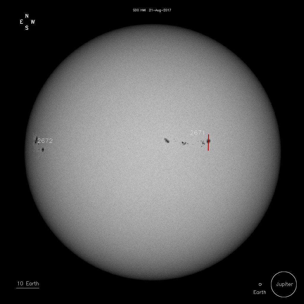
Il profilo spettrale

The spectral profile

Le differenze delle medie delle  tre misure delle due cuspidi a lato del centro riga ed il relativo d lambda sono state rispettivamente pari a:

The difference of the median of the three measures and related d lambda were:

Differenza           d lambda

  0.1408                 0.0704

  0.1534                0.0767

  0.1384                0.0692

E la loro media pari a

And their median of

 0.1442 A  ; d /lambda  0.0721 A

Quindi, applicando la formula precedente:

Then, applying the previous formula:

0.0721 x 10 ^13  =  1621 Gauss

   444886721

E l’errore:

And the error:

0.0767-0.0692/2= 0.0075 A, ovvero:

0.0075 x 10 ^13  =    169 Gauss

    444886721

Il valore alto dell’errore è attribuibile alla scarsa definizione della riga splittata verso il rosso ed alla conseguente difficoltà del software di ottenere il centro riga.

The high value of the error is probably due to the low definition of the splitted line toward the red and to the consequent difficulty of the software to get the center of the line

                                                        Quindi B= 1621 +-  169 Gauss

AR 2674 - 3 settembre 2017

La regione attiva 2674,un gruppo multipolare ben strutturato,con ombre piuttosto intense, come appariva nell'immagine SOHO-MDI del 3 settembre 2017, sicuramente uno dei più importanti (almeno sinora) del 2017 e con due componenti principali piuttosto estesi:

The active region 2674, a well-structured multipolar group, with rather intense umbras, as seen in the SOHO-MDI image of September 3, 2017, certainly (till now) one of the most important in 2017 and with two rather extensive components:

Un'immagine Hires  in luce H alpha del gruppo, presa da Fulvio Mete con un filtro Daystar Quark cromosphere

An Hires image of the group in H alpha light taken by Fulvio Mete by a Daystar Quark cromosphere filter

Ho cercato allora di valutare la forza magnetica delle due componenti principali del gruppo, che ho denominato A e B, come nella seguente immagine:la componente A appariva, oltre che più estesa, anche con un ombra più intensa della B.La comparazione tra le due costituiva quindi un interessante esperimento.

 I then tried to evaluate the magnetic strenght of the two main components of the group, which I called A and B, as in the following picture: Component A appeared, in addition to be a larger one, with a more intense shadow than B. Comparison between the two could be therefore an interesting experiment.

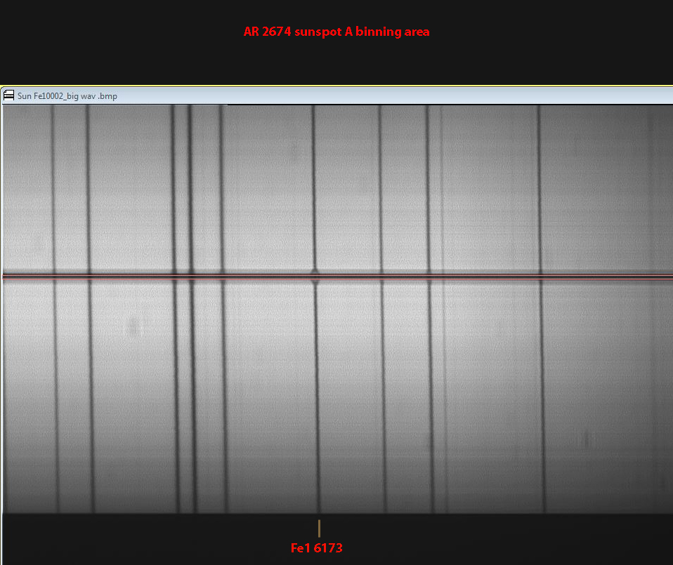
1- Componente A del gruppo

      component A of the group 

Lo spettro bidimensionale e l'area di binning:

Bidimensional spectrum and binning area

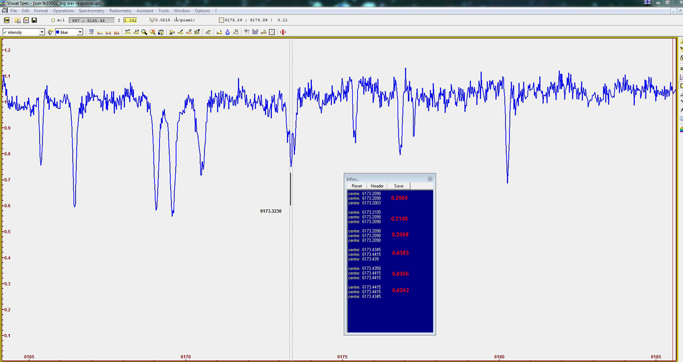
Il profilo spettrale: si notano tutte e tre le cuspidi delle righe Zeeman risultanti dalla scomposizione della Fe1 a 6173

The spectral profile: we clearly note all the three lines of the Zeeman splitting of the 6173 A Fe1 line.

Le differenze delle medie delle  tre misure delle due cuspidi a lato del centro riga ed il relativo d lambda sono state rispettivamente pari a:

The difference of the median of the three measures and related d lambda were:

Differenza           d lambda

  0.2317                 0.1158

  0.2296                0.1148

  0.2294                0.1147

E la loro media pari a

And their median of

 0.2302 A  ; d /lambda  0.1151 A

Quindi, applicando la formula precedente:

Then, applying the previous formula:

0.1151 x 10 ^13  =  2588 Gauss

   444886721

E l’errore:

And the error:

0.1158-0.1147/2= 0.00055 A, ovvero:

0.00055 x 10 ^13  =    12 Gauss

    444886721

Si può notare l'errore piuttosto esiguo,probabilmente merito del seeing notevole del giorno

We can note the low error, probably due to the excellent seeing of the day

Quindi B= 2588+- 12  Gauss

2- Componente B del gruppo

     Component B of the group 

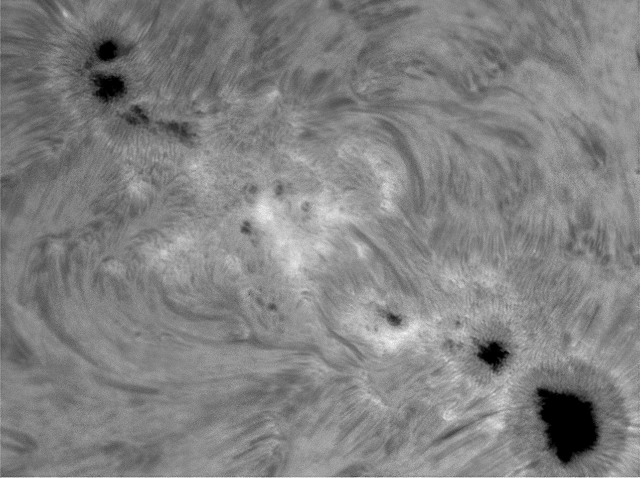
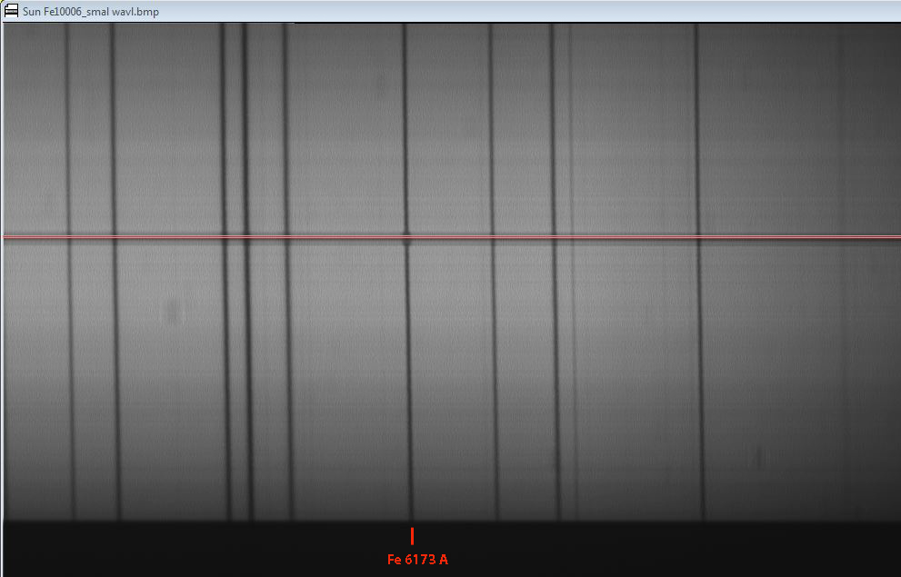
Lo spettro bidimensionale della componente B era molto meno intenso nello splitting Zeeman della riga, come si osserva nell'immagine:difficile dire a cosa questo sia attribuibile, ma una delle cause potrebbe essere quella che l'ombra della componente B, come si osserva dalle foto, era divisa in due parti, così sulla fenditura cadeva solo una delle due metà.

The bidimensional  spectrum showed a more less intense Zeeman splitting of the Iron line: difficult to say the cause of this; may be the structure of component B, whose umbra, as you can see from the photos, was divided in two parts, so the slit covered only one of the two.

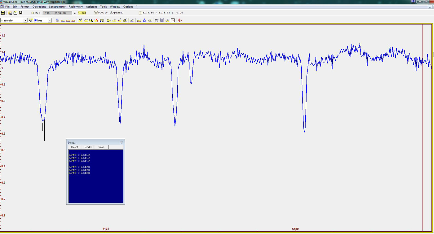
La conseguenza era che VSpec non riusciva a separare nettamente le righe Zeeman,come si osserva nell'immagine del profilo, nè tantomeno ad indicarne i centri.Sono tuttavia riuscito ad ottenere i soli centri riga della parte centrale e di quella rivolta verso il rosso, misurandone il valore.

The consequence was that VSpec wasn't able to split clearly the Zeeman lines, but only (and hardly) the two  of  the center and of that toward the red, measuring their value.

La differenza in Angstrom era quindi direttamente pari al d lambda, e risultava di  0.3858-0.3232 = 0.0626.Era quindi

The difference in Angstrom resulted to be than equal to the d lambda and of  0.3858-0.3232 = 0.0626.Was then:

0.0626 x 10 ^13  =   1407  Gauss

    444886721

Non essendo possibile valutare l'errore,

Not being possible to evaluate the error            B= 1407 Gauss

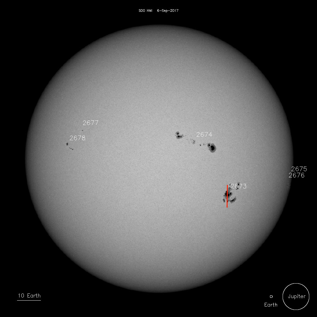
AR 2673 - 6 settembre 2017

Ci si potrebbe chiedere come mai con questo gruppo si sia interrotta la sequenza numerico-  temporale delle macchie del 2017, nel senso che, pur avendo una numerazione inferiore alla precedente sia stata ripresa successivamente a questa, tre giorni dopo.La risposta è facile: in tre giorni, dal 3 al 6 settembre 2017, mentre la 2674 non ha presentato grossi cambiamenti, la 2673 ha segnato uno sviluppo veramente notevole ,direi quasi eccezionale come si può notare nell'immagine che segue (fonte Soho-MDI).

One might wonder why with this group the number-time sequence of the sunspots of 2017 was interrupted, meaning that while having a number smaller than the previous one was taken later than this, three days later. The answer is easy: in three days, from September 3 to September 6, 2017, while 2674 did not make any major changes, 2673 marked a truly remarkable development, I would say almost as exceptional as can be seen in the following picture (source Soho-MDI).

Ciò ha prodotto un top di attività, microflares, flares e via dicendo,sino ad arrivare ad un flare di forza M 8.1 l'8 settembre 2017, quando era prossima al lato ovest del disco solare.Nell'immagine sottostante una ripresa Halpha di Fulvio Mete il giorno 4 settembre 2017, quando la 2673 stava iniziando la sua notevole ascesa di potenza ed estensione.

This produced a top of activity,  a microflares, flares and so on,culminating in a M8.1 on september, 8, 2017, when it was approaching to the western limb.In the following image, a shot in H alpha light of Fulvio Mete, on september,4 2017, when the 2673 begun its noticeable rise of strenght and extension.

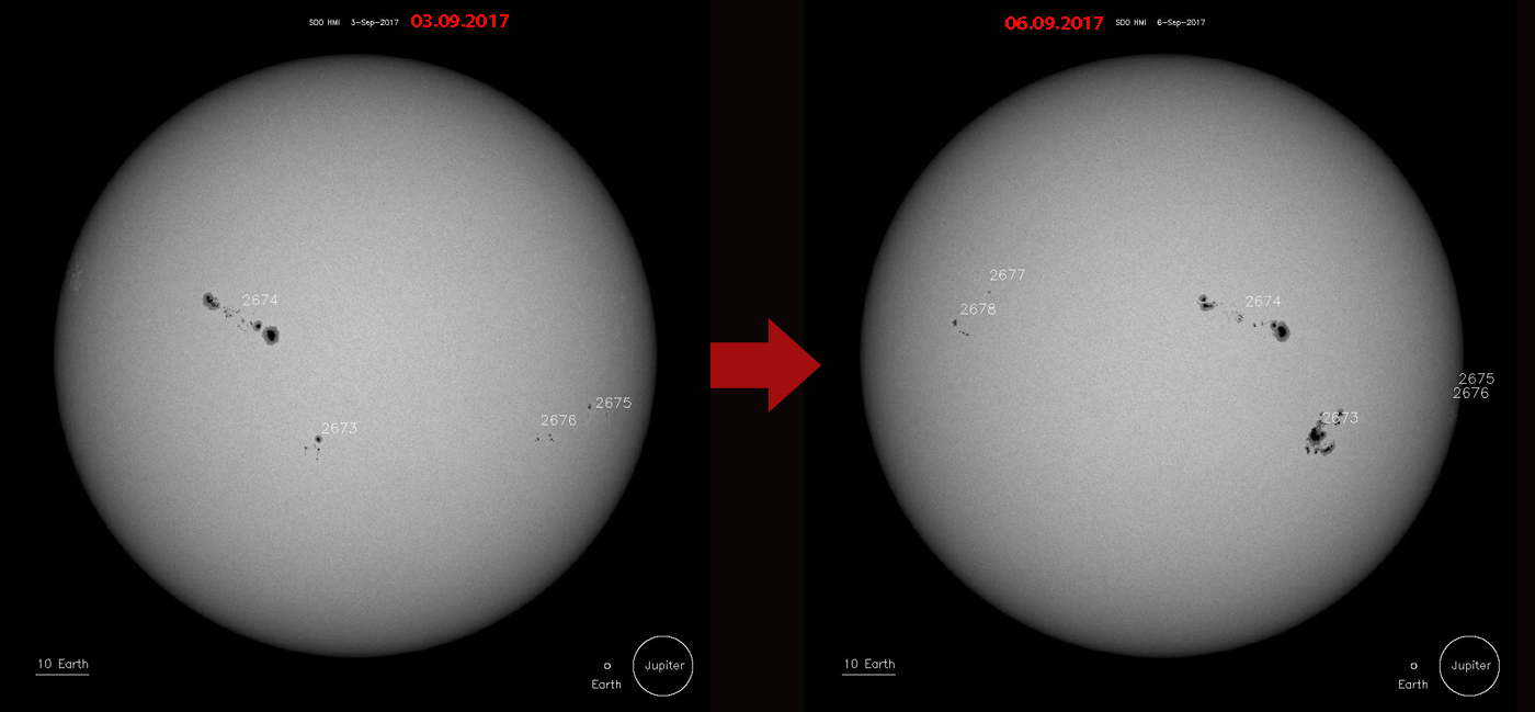
Il 6 settembre, data della ripresa spettroscopica della macchia, questa era prossima al culmine della sua forza, e presentava il seguente spettro bidimensionale, con indicata l'area di binning sulla quale è stato ricavato il profilo:  

On september, 6, date of spectroscopic shot of the sunspot, it showed the following two-dimensional spectrum, on which is indicated the binning area

Come si può osservare sopra e sotto la macchia centrale si notano gli effetti delle altre due componenti del gruppo.E' bene precisare che la misura del campo magnetico ha riguardato la sola ombra della macchia principale del gruppo, sulla quale era puntata la fenditura, come si osserva nell'immagine del disco solare che segue .E' stata, inoltre, usata per l'acquisizione dei filmati (sei in tutto, dei quali si è scelto il migliore con lo stacking di 400 frames) una camera IS DMK 51 di risoluzione maggiore, 1600 x 1200 pixel  contro i 1280x 960 della DMK 41  normalmente usata, ma di sensibilità lievemente inferiore.In conseguenza la dispersione spettrale è stata di 0.0200 A/pix anzichè gli usuali 0.0215.

As you can see above and below the central spot, you can notice the effects of the other two components of the group. It is worth pointing out that the magnetic field measurement was only the umbra of the group's main spot on which the slit was pointed, as it is observed in the image of the following solar disc. It was also used to capture the videos (six of them were the best one with 400 frames stacking) an IS DMK 51  camera of resolution  1600 x 1200 pixels larger than the DMK 41 1280x 960 normally used but with slightly lower sensitivity. As a result spectral dispersion was 0.0200 A / pix instead of the usual 0.0215.

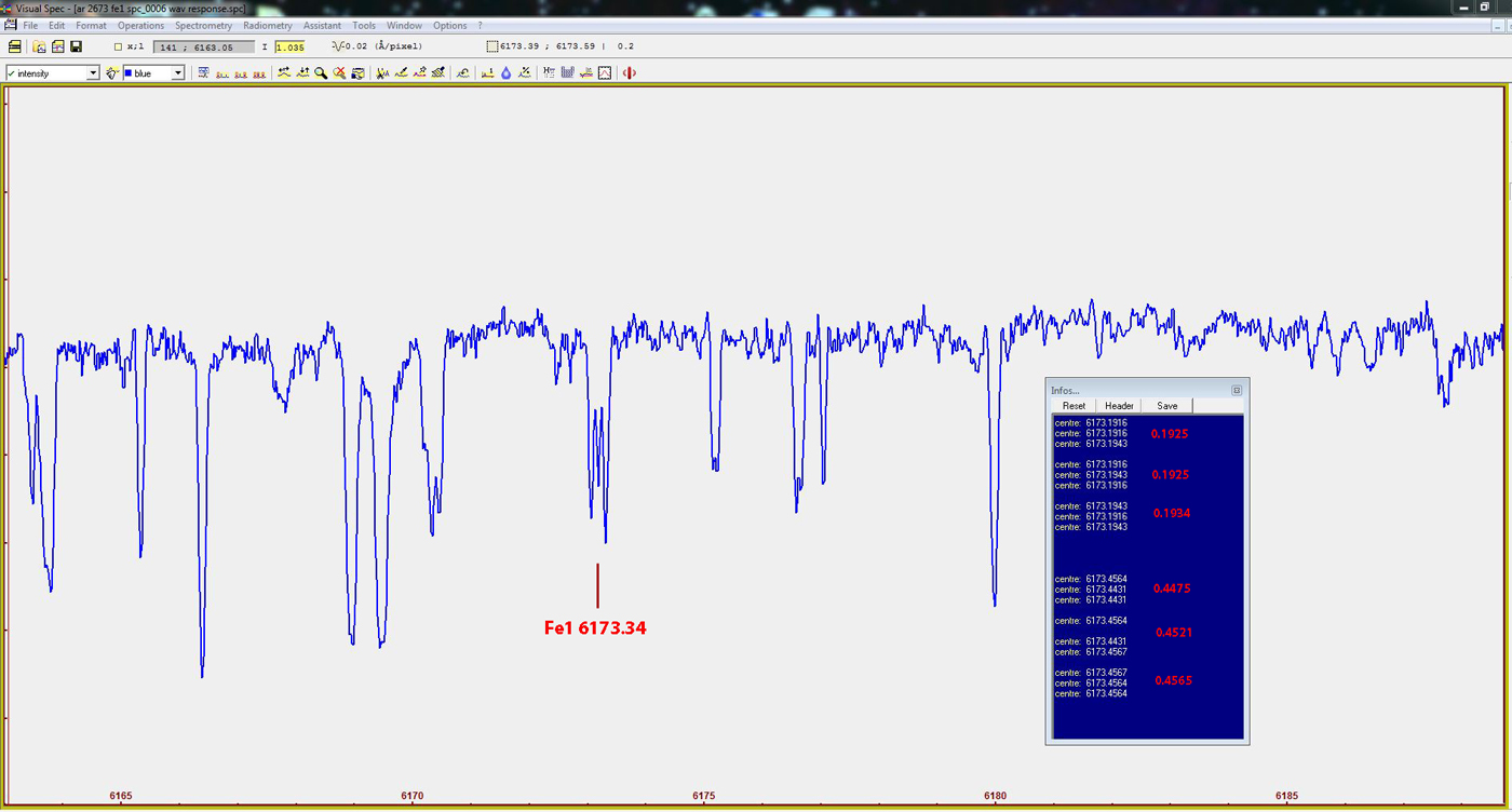
Le differenze delle medie delle  tre misure delle due cuspidi a lato del centro riga ed il relativo d lambda sono state rispettivamente pari a:

The difference of the median of the three measures and related d lambda were:

Differenza           d lambda

  0.2550                0.1275

  0.2596                0.1298

  0.2631               0.1315

E la loro media pari a

And their median of

 0.2592 A  ; d /lambda  0.1296 A

Quindi, applicando la formula precedente:

Then, applying the previous formula:

0.1296 x 10 ^13  =  2913 Gauss

   444886721

E l’errore:

And the error:

0.1315-0.1275/2= 0.002 A, ovvero:

0.002 x 10 ^13  =    45 Gauss

    444886721

Quindi B= 2913 +-  45 Gauss

AR 2683 - 30 settembre 2017

Un'altra macchia di medie dimensioni,monopolare divisa da un light bridge, che ha contraddistinto insieme alle altre una seconda metà dell'anno  con un inaspettato livello di attività rispetto al semestre precedente.

Another sunspot of medium extension, with a light bridge, which,with the others, has  featured  in the second half of the year an  unexpected increase of activity respect to the previous half year.

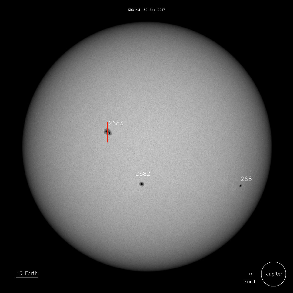
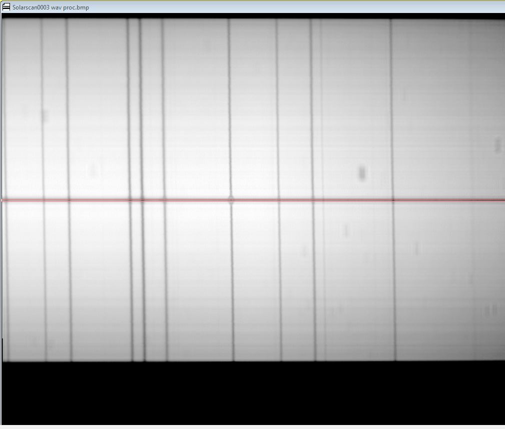
Stavolta ho dovuto effettuare uno stretching lineare sull'immagine dello spettro bidimensionale per schiarire l'ombra ed evidenziare lo splitting della riga nell'ombra.

This time I had to perform a linear stretching on the two dimensional spectrum to make evident the splitting of the line in the umbra

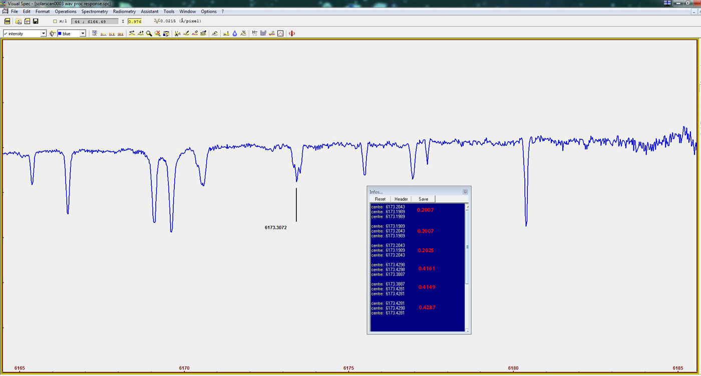
Le differenze delle medie delle  tre misure delle due cuspidi a lato del centro riga ed il relativo d lambda sono state rispettivamente pari a:

The difference of the median of the three measures and related d lambda were:

Differenza           d lambda

  0.2154                0.1077

  0.2142                0.1071

  0.2262               0.1131

E la loro media pari a

And their median of

 0.2186 A  ; d /lambda  0.1093 A

Quindi, applicando la formula precedente:

Then, applying the previous formula:

0.1093 x 10 ^13  =  2457 Gauss

   444886721

E l’errore:

And the error:

0.1131-0.1071/2= 0.003 A, ovvero:

0.003 x 10 ^13  =    67 Gauss

    444886721

Quindi B= 2457+-  67 Gauss